Support vector machines do not always separate linearly separable data in classification tasks
Support vector machines
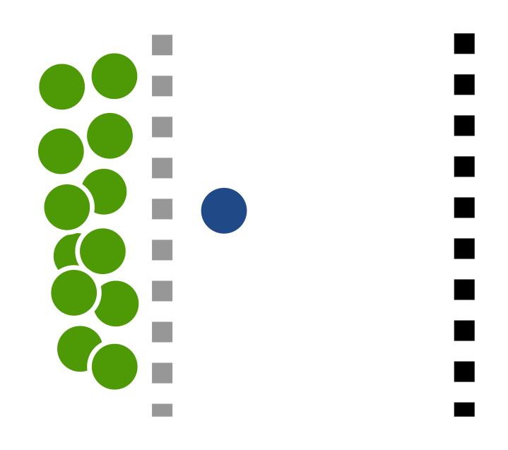
Support vector machines (SVMs) are all about separating linearly separable data. Here is a simple example of an SVM failing to separate linearly separable data in 1D. I thought this example was quite insightful.
In general a linear SVM tries to minimize
where we define the slack variables
with \(f(x) = w^t x + b\) the classification rule and \(y_i \in \{-1, 1\}\) the training labels.
A pathological example
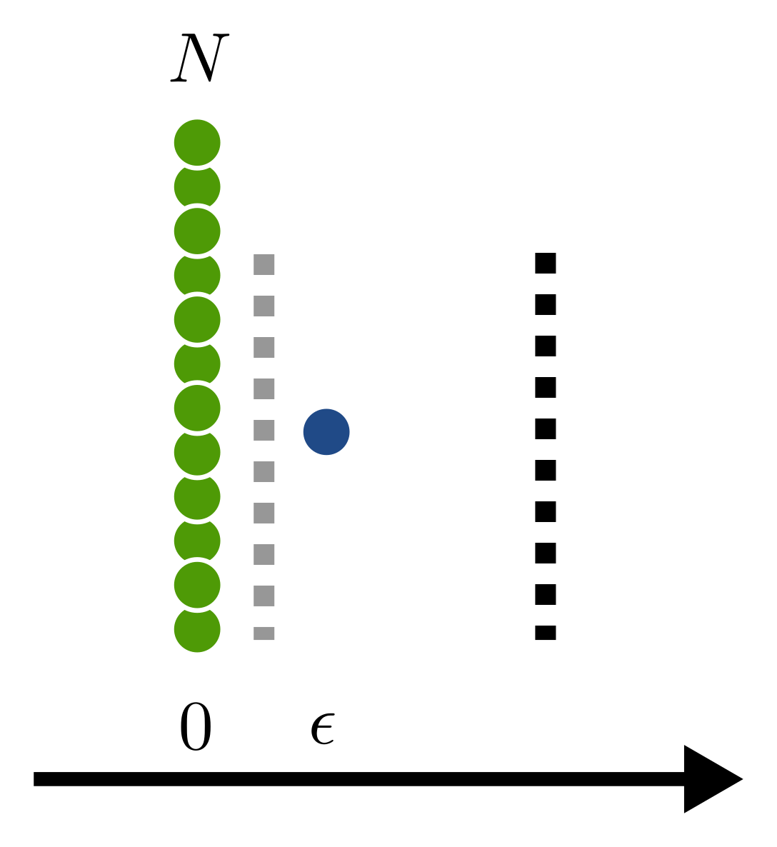
Now consider the following example: We have \(N\) data points of class \(-1\) located at \(0\) and \(1\) data point of class \(+1\) located at \(\epsilon > 0\). We will now prove, that the optimal SVM, for \(\epsilon\) small enough and \(N\) large enough does not separate the classes.
First, some intuition. The loss function \(J\) is a trade-off between a large margin for class separation (that is the \(\|w\|_2^2\) term) and avoidance of classification errors (that is the \(C \sum \ldots\) term). To avoid classification errors \(w\) will have to be large. The magnitude of \(w\) will have to scale with \(1/\epsilon\) and will therefore increase as \(\epsilon\) decreases. On the other hand, a small \(w\) will result in larger classification errors. These errors will scale with \(N\). So for large \(N\) and small \(\epsilon\) a linearly separating SVM should produce a large value of \(J\).
Now, let's prove that rigorously. We first derive an upper bound on the optimal \(J\) value. Any specific value of \((w,b)\) constitutes such an upper bound. Clearly
for \(\epsilon\) small enough. The SVM given through \((w,b) = (1, -1)\) does clearly not separate the classes. We now proceed to show, that any SVM linearly separating the classes has larger \(J\) than our SVM above. The SVM above is also clearly not optimal. But if our suboptimal SVM above beats any SVM which linearly separates the classes, then every linearly separating SVM is also beaten by the optimal SVM.
For a separating SVM, we have the two conditions
or equivalently
We look at the minimum in the two regions \(b \leq -1\) and \(-1 < b < 0\). So that
For \(b \leq -1\) we find.
The first inequality holds since we just ignored the positive terms from the slack variables. The last inequality holds as \(b=-1\) minimizes \(b^2\) in that region. We already see, that \(J\) gets really large in this region if \(\epsilon\) is really small. We require a large \(w\) to separate close by points by a large margin.
Let's check the other region \(-1 < b < 0\). We have
The first inequality holds as we just ignored the error term from the point at \(\epsilon\). The second equality holds as the minimum of \(w\) really only applies to the first term as this is the only term depending on \(w\). Moreover, since \(-1 < b < 0\), we could drop the absolute value. The following inequality holds as taking the minimum over all of \(\mathbb{R}\) only decreases the minimum. The last equality follows as taking the derivative with respect to \(b\) and setting it to zero yields \(b=-CN\epsilon^2\).
You might be (rightfully) worried that the last term is negative. But, e.g. for \(\epsilon=1/\sqrt{N}\) and \(C = 1\) we get \(1- CN\epsilon^2=0\) and therefore [1]
So we see that also this blows up if \(N\) is large enough. Therefore, the optimal SVM does not separate the classes although they are linearly separable.
This behavior really depends on the value of \(C\). As \(C\) increases classification errors are punished more and a smaller classification margin is tolerated. Hence, for \(C\) large enough, the classes will be separated. However, for small \(C\), classification errors are less expensive but a small margin is punished more. Therefore, the optimal solution might has a larger margin at the cost of some misclassifications.
Cute, isn't it?
| [1] | we then have \(b=-1\) |